“Give more than you planned to”
Principal Concepts
Must be able to explain concretely and concisely
- P value, significance level, confidence level, confidence interval
- Common Distirbutions (pdf, mean, variance): Normal, Binomial, Bernoulli, Geometric, Poisson, Exponential
- Central limit theroem and it’s underlying assumption
- Law of large number
- Hypothesis testing and how to calculate the sample size for hypothesis testing
- Estimator vs. estimate
- Simpson’s Paradox and correction formula
- Bias-variance trade off
- ANOVA
- Bootstrap
- Type 1 and type 2 error
- Percision vs. recall
- Z test and T test (formula, underlying assumption)
- Bayesian formula for conditional probability
OLS
OLS is a type of parameter estimation methods for estimating the unknown parameters in a linear regression model by minimizing the sum of the squares of the differences between the observed response variable and predicted response variable.
Assumptions for Linear Regression model
- the mean of the error term is 0 (Unbiasedness)
- variables are linearly related
- the variance of the error term is constant
- error values are independent and normally distributed (Ensures that all the (Xi, Yi) are drawn randomly from the sample population)
- x variables are not too highly correlated (collinearity/multicollinearity)
- x values are fixed and are measured without error. From 1point 3acres bbs
Solutions to violations of assumptions (less robustness)
- Transformation
- Use weighted least squares, generalized least squares, lasso/ridge regression
Assumptions for Logistic Regression model
- Explanatory variables are measured without error
- Model is correctly specified (neither over fitting nor under fitting, all important variables included, etc.)
- Outcomes not completely linearly separable (i.e. x values cannot completely determine whether y = 0 or y = 1, make parameter estimates unstable). From 1point 3acres bbs
- Observations are independent
-
It requires large sample size, n
Because of MLE, it requires more observations than usual regression, especially if one of the categories occurs rarely (rule of thumb: at least 10 obs for each outcome (0/1))
- Collinearity/multicollinearity
The difference between linear regression and logistic regression
- Linear regression is used when the dependent variable is continuous and logistic regression is used when dependent variable is binary.
- Linear regression uses OLS and Logistic regression uses Maximum Likelihood method to estimate coefficients
R-squared
How much of the variation in Y can be explained by the X Every time we add a variable to the regression, the R-squared value will stay the same or increase, even if the variable is not helpful. So the Adjusted R-squared can be adjusted for the numbers of variables.
Outlier
Scatterplot, Boxplot, Z-score
Solutions 1. transformation 2. different model
Collinearity/Multicollinearity-baidu 1point3acres
Two or more explanatory variables are moderately/highly correlated with each other.
When independent variables are correlated, it indicates that changes in one variable are associated with shifts in another variable. The stronger the correlation, the more difficult it is to change on variable without changing another. It becomes difficult for the model to estimate the relationship between each independent variable and dependent variable.
Detecting Multicollinearity
- Look at the scatterplot and correlation matrices
- VIF, variance inflation factor, VIF > 10
Solutions
- Drop one or more explanatory variables from the final model
- Center/standardize independent variables to reduce the effects of multicollinearity (Transformation)
- Use ridge regression to reduce issues
What’s the difference between Type I and Type II error?
Type I error is the rejection of a true null hypothesis
Type II error is failing to reject a false null hypothesis
Z-score (critical value)
How far the value measured from the mean, in terms of standard deviation (population variance is known) \(\bf{Z} = \frac{\bar{X} - \mu}{\sigma} \sim\mathbf{N}(\mathbf{0},\mathbf{1})\)
\(\mu\)
- hypothesized population mean
t-statistic
It’s the ratio of the departure of the estimated value of a parameter from its hypothesis testing (population variance is unknown), when n = 30, t is a close form of normal distribution
\(t = \frac{\bar{X} - \mu}{s/\sqrt n} , \mu\) - hypothesized population mean
Hypothesis Testing
It’s a method of statistical inference that tests the usefulness of X as a predictor of Y.
P-value
It’s the probability of getting the observed value of the test statistic, or a value with even greater evidence against H_0, if the null hypothesis is true.
Correlation measures the strength of a linear association.
If the relationship between X and Y cannot be described by a line, then correlation is meaningless. You should always check a scatter plot to see if X and Y have a linear relationship before using statistic r Correlation does not imply causation, it measures the strength of a linear association: If X and Y have a high correlation, it does not tell you anything about whether X causes Y or whether Y causes X.
In-sample prediction VS Out-of-sample prediction
In-sample prediction is prediction of y from x which is in the range of the data Out-of-sample prediction of y from x is outside of the range of the data, it’s dangerous because you don’t know whether the linear relationship holds in regions where you don’t have data
Model Evaluation
- MSE (Mean Square Error): Estimate variability of response variable around the regression line
- R-squared Value
Variable Selection Criteria
The model containing all of the predictors will always have the smallest MSE and largest R-squared Value. (So MSE and R-squared value are not applicable to select the best model)
- Adj R-squared Value
- Cp, BIC, AIC
Parametric/non-parametric Models
In a parametric model, you know which model exactly you will fit to the data, e.g., linear regression line. In a non-parametric model, however, the data tells you what the ‘regression’ should look like.
Lasso and Ridge
Ridge and Lasso regression uses two different penalty functions. The key difference between these techniques is that Lasso shrinks the less important feature’s coefficient to zero but Ridge won’t. In ridge regression, the penalty is the sum of the squares of the coefficients and for the Lasso, it’s the sum of the absolute values of the coefficients. The constraint region for ridge is the disk, while that for lasso is a diamond. Both methods find the first point where the elliptical contours hit the constraint region. Unlike the disk (ridge), the diamond (lasso) has corners, if the solution occurs at a corner, then it has one parameter equal to zero (shrink to zero).
Heteroscedasticity
In linear regression modes, Heteroscedasticity refers to a circumstance that the residuals (errors) change across values of an explanatory variable. -baidu 1point3acres
CLT
The central limit theorem states that if you have a population with mean μ and standard deviation σ and take sufficiently large random samples from the population with replacement, then the distribution of the sample means will be approximately normally distributed. This will hold true regardless of whether the source population is normal or skewed, provided the sample size is sufficiently large (usually n > 30). If the population is normal, then the theorem holds true even for samples smaller than 30. This means that we can use the normal probability model to quantify uncertainty when making inferences about a population mean based on the sample mean.
Unbiased Estimator
θ is a population parameter and \hat{\theta} is an estimator, we hope theta hat is a good way of estimating θ. \hat{\theta} is a random variable because each time we take a sample, we will get a different estimate of θ, therefore we can determine the bias of an estimator is E(\hat{\theta} ) - θ. Hence, an unbiased estimator is where the bias equals 0 which indicates that the average of \hat{\theta} across repeated samples equals the true value of θ regardless of sample size n.
MLE
We seek estimates for θ such that the predicted probability p(x_i) for each individual observation corresponds as closely as possible to the observed individual’s value. (Yield a number close to one for all individuals who defaulted, a number close to zero for all individuals who don’t).
MLE, it selects as estimates the values of the parameters that maximize the likelihood (the joint probability function or joint density function) of the observed sample.
Variance and Covariance
Variance refers to the spread of a data set around its mean value, while a covariance refers to the measure of the directional relationship between two random variables.
Confidence and Prediction Intervals
Confidence intervals estimates the theoretical mean of Y at a given value of X.
Prediction intervals predicts a single value of Y at a given value of X.
There is extra variability in the prediction of a single value, as opposed to estimating the mean of all values at that point, so the prediction intervals are wider than confidence intervals.
Welch’s t-test
In statistics, Welch’s t-test, or unequal variances t-test, is a two-sample location test which is used to test the hypothesis that two populations have equal means. It is named for its creator, Bernard Lewis Welch, and is an adaptation of Student’s t-test,[1] and is more reliable when the two samples have unequal variances and/or unequal sample sizes.[2][3] These tests are often referred to as “unpaired” or “independent samples” t-tests, as they are typically applied when the statistical units underlying the two samples being compared are non-overlapping. Given that Welch’s t-test has been less popular than Student’s t-test[2] and may be less familiar to readers, a more informative name is “Welch’s unequal variances t-test” — or “unequal variances t-test” for brevity
Student’s t test
Independent two-sample t-test
Equal sample sizes, equal variance
Given two groups (1, 2), this test is only applicable when:
the two sample sizes (that is, the number n of participants of each group) are equal;
it can be assumed that the two distributions have the same variance;
Violations of these assumptions are discussed below.
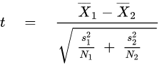
The t statistic to test whether the means are different can be calculated as follows:


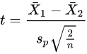
OR
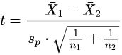
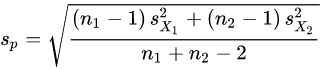


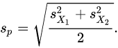
Here sp is the pooled standard deviation for n = n1 = n2 and s 2
X1 and s 2 X2 are the unbiased estimators of the variances of the two samples.
Degree of Freedom
Imagine you’re a fun-loving person who loves to wear hats. You couldn’t care less what a degree of freedom is. You believe that variety is the spice of life.
Unfortunately, you have constraints. You have only 7 hats. Yet you want to wear a different hat every day of the week.
7 hats
On the first day, you can wear any of the 7 hats. On the second day, you can choose from the 6 remaining hats, on day 3 you can choose from 5 hats, and so on.
When day 6 rolls around, you still have a choice between 2 hats that you haven’t worn yet that week. But after you choose your hat for day 6, you have no choice for the hat that you wear on Day 7. You must wear the one remaining hat. You had 7-1 = 6 days of “hat” freedom—in which the hat you wore could vary!
That’s kind of the idea behind degrees of freedom in statistics. Degrees of freedom are often broadly defined as the number of “observations” (pieces of information) in the data that are free to vary when estimating statistical parameters.
Expected Value or Expectation vs Avg or Mean
The concept of expectation value or expected value may be understood from the following example. Let X represent the outcome of a roll of an unbiased six-sided die. The possible values for X are 1, 2, 3, 4, 5, and 6, each having the probability of occurrence of 1/6. The expectation value (or expected value) of X is then given by
(X)expected=1(1/6)+2⋅(1/6)+3⋅(1/6)+4⋅(1/6)+5⋅(1/6)+6⋅(1/6)=21/6=3.5
Suppose that in a sequence of ten rolls of the die, if the outcomes are 5, 2, 6, 2, 2, 1, 2, 3, 6, 1, then the average (arithmetic mean) of the results is given by
(X)average=(5+2+6+2+2+1+2+3+6+1)/10=3.0
We say that the average value is 3.0, with the distance of 0.5 from the expectation value of 3.5. If we roll the die N times, where N is very large, then the average will converge to the expected value, i.e.,(X)average=(X)expected. This is evidently because, when N is very large each possible value of X (i.e. 1 to 6) will occur with equal probability of 1/6, turning the average to the expectation value.
Unequal size ab testing
Use Welch’s t-test
If the variances of the metric of interest for A and B are similar (typically the case), your test sensitivity will be dominated by the smaller sample size. Running equally-sized variants (A and B) is therefore optimal for variance reduction, and hence running 50/50% is the most efficient from a statistical power perspective.
If you’re properly randomizing signed-in users and these users are reasonably independent (i.e. you don’t expect them to talk to each other about the experience that is being varied), then using unequal size groups is fine: sample means are unbiased estimators of population means, so the group size cannot introduce any bias. However, your p-values (confidence levels) will be more accurate if you use exact statistical tests like Fisher’s Test for rates and the Mann-Whitney U Test for continuous outcomes instead of Student’s T-Test or Welch’s T-Test, especially for smallish samples like 8000.
How to assess the statistical significance
is this insight just observed by chance or is it a real insight?
Statistical significance can be accessed using hypothesis testing:
-
Stating a null hypothesis which is usually the opposite of what we wish to test (classifiers A and B perform equivalently, Treatment A is equal of treatment B)
-
Then, we choose a suitable statistical test and statistics used to reject the null hypothesis
-
Also, we choose a critical region for the statistics to lie in that is extreme enough for the null hypothesis to be rejected (p-value)
-
We calculate the observed test statistics from the data and check whether it lies in the critical region
Common tests:
-
One sample Z test
-
Two-sample Z test
-
One sample t-test
-
paired t-test
-
Two sample pooled equal variances t-test
-
Two sample unpooled unequal variances t-test and unequal sample sizes (Welch’s t-test)
-
Chi-squared test for variances
-
Chi-squared test for goodness of fit
-
Anova (for instance: are the two regression models equals? F-test)
-
Regression F-test (i.e: is at least one of the predictor useful in predicting the response?)
Importance in classification and regression
-
Skewed distribution
-
Which metrics to use? Accuracy paradox (classification), F-score, AUC
-
Issue when using models that make assumptions on the linearity (linear regression): need to apply a monotone transformation on the data (logarithm, square root, sigmoid function…)
-
Issue when sampling: your data becomes even more unbalanced! Using of stratified sampling of random sampling, SMOTE (“Synthetic Minority Over-sampling Technique”, NV Chawla) or anomaly detection approach
Central Limit Theorem
The CLT states that the arithmetic mean of a sufficiently large number of iterates of independent random variables will be approximately normally distributed regardless of the underlying distribution. i.e: the sampling distribution of the sample mean is normally distributed.
-
Used in hypothesis testing
-
Used for confidence intervals
-
Random variables must be iid: independent and identically distributed
-
Finite variance
sequential analysis or sequential testing
In statistics, sequential analysis or sequential hypothesis testing is statistical analysis where the sample size is not fixed in advance. Instead data are evaluated as they are collected, and further sampling is stopped in accordance with a pre-defined stopping rule as soon as significant results are observed. Thus a conclusion may sometimes be reached at a much earlier stage than would be possible with more classical hypothesis testing or estimation, at consequently lower financial and/or human cost.