“Hope for the best and prepare for the worst”
Let’s take a look at why LSTM solves problem of gradient vanishing of RNN.
Jump here for details of LSTM avoid gradient vanishing
LSTM (Long Short-Term Memory)
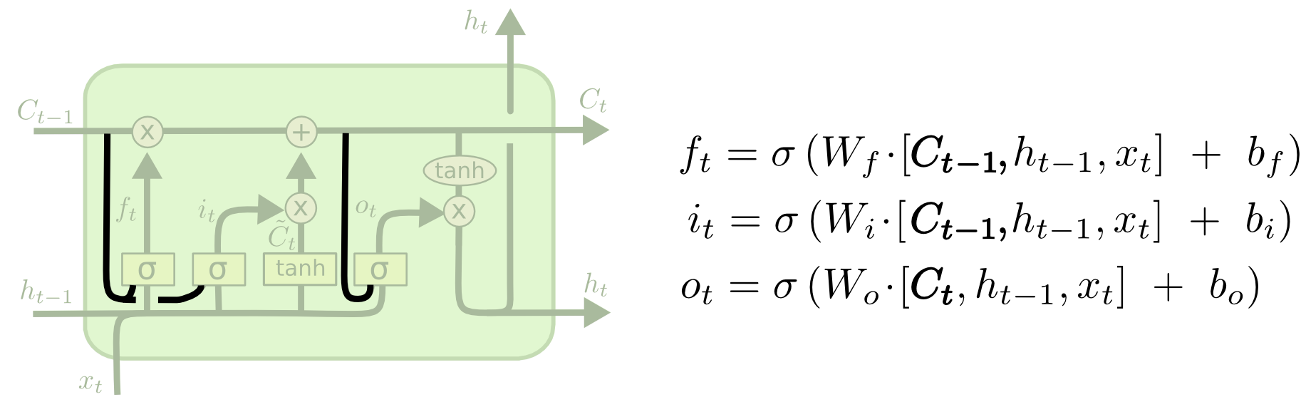
Gates
Forget gate
This gate decides what information should be thrown away or kept, The closer to 0 means to forget, and the closer to 1 means to keep.
Input Gate
To update the cell state (memory pipeline); decides what information is relevant to add from the current step
Output Gate
The output gate decides what the next hidden state should be
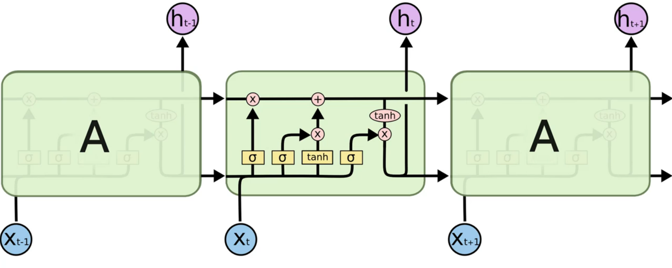
Architecture
- Decide what information we’re going to throw away from the cell state (forget gate, value range from 0-1 by sigmoid)
- Decide what new information we’re going to store/add in the cell state ;
- a sigmoid layer called the “input gate layer” decides which values we’ll update.
- a tanh layer creates a vector of new candidate values, C~t, that could be added to the state
- Decide what we’re going to output
- First, we run a sigmoid layer which decides what parts of the cell state we’re going to output. Then, we put the cell state through tanh (to push the values to be between −1 and 1) and multiply it by the output of the sigmoid gate, so that we only output the parts we decided to.
Avoid gradient vanishing HOW?
- By turning the multiplication to additive
Weight matrix are no longer multiplication, instead, cell state is adding the previous information and current processed information and pass through.
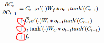
- Gates functions
If we start to converge to zero (gradient vanishing/above function), we can always set the values of f_t (and other gate values) to be higher in order to bring the value of

closer to 1, thus preventing the gradients from vanishing (or at the very least, preventing them from vanishing too quickly). One important thing to note is that the values f_t, sigma_t, i_t, and ˜C_t are things that the network learns **to set (conditioned on the current input and hidden state). Thus, in this way the network learns to decide **when** **to let the gradient vanish, and when to preserve it, by setting the gate values accordingly!
Summary: Two main things to answer why and how:
- The additive update function for the cell state gives a derivative that’s much more ‘well behaved’
- The gating functions allow the network to decide how much the gradient vanishes, and can take on different values at each time step. The values that they take on are learned functions of the current input and hidden state.
Why use Tanh and Sigmoid
- The sigmoid (0 - 1) layer tells us which (or what proportion of) values to update and the tanh (-1 - 1) layer tells us how to update the state (increase or decrease)
- The output from tanh can be positive or negative, determining whether increases and decreases in the state.
- After the addition operator the absolute value of c(t) is potentially larger than 1. Passing it through a tanh operator ensures the values are scaled between -1 and 1 again, thus increasing stability during back-propagation over many timesteps.
Tanh and sigmoid have
- Well defined gradient at all points
- They are both easily converted into probabilities. The sigmoid is directly approximated to be a probability. (As its 0-1); Tanh can be converted to probability by (tanh+1)/2 will be between 0-1
- Well defined thresholds for classes. -> tanh-> 0 and sigmoid -> 0.5
- They can both be used in calculating the binary crossentropy for classification
LSTM Variations
- * This means that we let the gate layers look at the cell state. The above diagram adds peepholes to all the gates, but many papers will give some peepholes and not others.
- * We only forget when we’re going to input something in its place. We only input new values to the state when we forget something older.
- * Cheaper computational cost * 3 gates vs 2 gates in gru * no ouput gate, no second non linearity and they don’t have memory ct it is same as hidden state in gru. * **update gate** in gru does the work of **input and forget gate in lstm.**

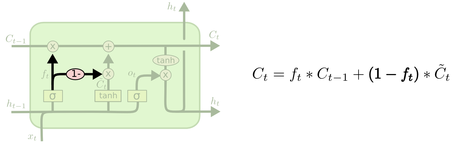
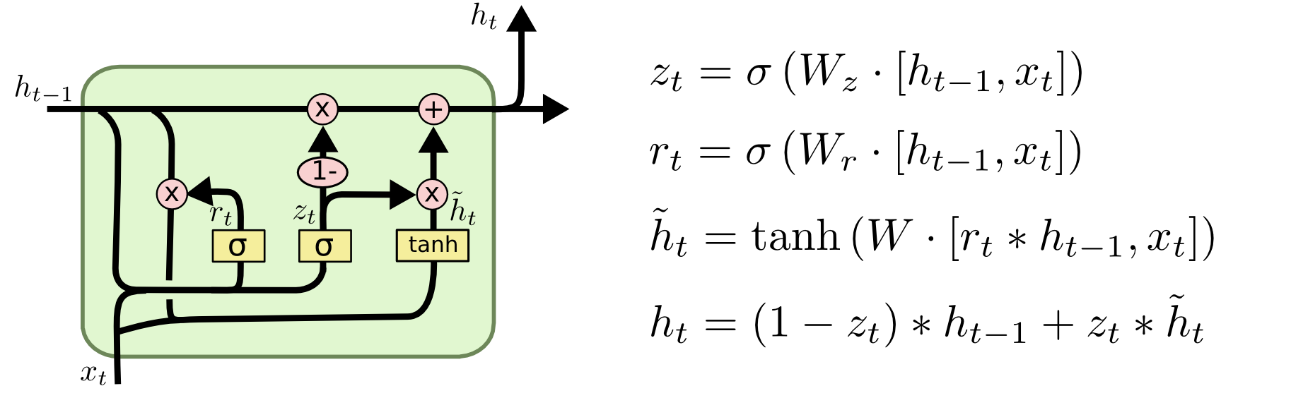
Why “1-“ in output gate
Instead of doing selective writes and selective forgets, we define forget as 1 minus write gate. So whatever is not written is forgotten.
Standardisation vs Normalisation
Timestep
60 timesteps of the past information from which our RNN is gonna try to learn and understand some correlations, or some trends, and based on its understanding, it’s going to try to predict the next output.
Too small number will cause overfitting
Improve RNN
- Getting more training data: we trained our model on the past 5 years of the Google Stock Price but it would be even better to train it on the past 10 years.
- Increasing the number of timesteps: the model remembered the stock prices from the 60 previous financial days to predict the stock price of the next day. That’s because we chose a number of 60 timesteps (3 months). You could try to increase the number of timesteps, by choosing for example 120 timesteps (6 months).
- Adding some other indicators: if you have the financial instinct that the stock price of some other companies might be correlated to the one of Google, you could add this other stock price as a new indicator in the training data.
- Adding more LSTM layers: we built a RNN with four LSTM layers but you could try with even more.
- Adding more neurones in the LSTM layers: we highlighted the fact that we needed a high number of neurones in the LSTM layers to respond better to the complexity of the problem and we chose to include 50 neurones in each of our 4 LSTM layers. You could try an architecture with even more neurones in each of the 4 (or more) LSTM layers.
Resources
LSTM solves problem of gradient vanishing