“The value of life lies not length of days, but in the use of we make of them”
This post aims to review some concepts of machine learning, statistics, probability for data scientist interview. Big welcome to comment below to correct my inappropriate interpretation.
Updating…
Machine learning
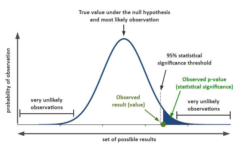
P value
Probability of observing a sample “more extreme” than the ones observed in your data assuming H0 is true.
Power
The power of a binary hypothesis test is the probability that the test rejects the null hypothesis when a specific alternative hypothesis is true.
sensitivity of a binary hypothesis test
Probability that the test correctly rejects the null hypothesis H0 when the alternative is true H1
Ability of a test to detect an effect, if the effect actually exists
Power=P(rejectH0|H1istrue)
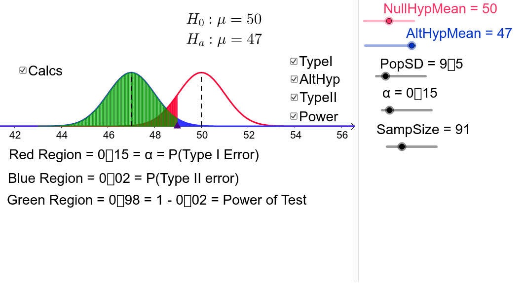
As power increases, chances of Type II error (false negative) decrease
Used in the design of experiments, to calculate the minimum sample size required so that one can reasonably detects an effect. i.e: “how many times do I need to flip a coin to conclude it is biased?”
Used to compare tests. Example: between a parametric and a non-parametric test of the same hypothesis
Confidence interval
More strictly speaking, the confidence level represents the frequency (i.e. the proportion) of possible confidence intervals that contain the true value of the unknown population parameter.
Significance level
A 5% significance level means that if you declare a winner in your AB test (reject the null hypothesis), then you have a 95% chance that you are correct in doing so. It also means that you have significant result difference between the control and the variation with a 95% “confidence.” This threshold is, of course, an arbitrary one and one chooses it when making the design of an experiment.
Test power
The probability of detecting that difference between the original rate and the variant conversion rates.
Unequal sample sizes AB test
If you’re properly randomizing signed-in users and these users are reasonably independent (i.e. you don’t expect them to talk to each other about the experience that is being varied), then using unequal size groups is fine: sample means are unbiased estimators of population means, so the group size cannot introduce any bias. However, your p-values (confidence levels) will be more accurate if you use exact statistical tests like Fisher’s Test for rates and the Mann-Whitney U Test for continuous outcomes instead of Student’s T-Test or Welch’s T-Test, especially for smallish samples like 8000.
Cross Validation
Cross-validation, sometimes called rotation estimation,[1][2][3] or out-of-sample testing is any of various similar model validation techniques for assessing how the results of a statistical analysis will generalize to an independent data set. It is mainly used in settings where the goal is prediction, and one wants to estimate how accurately a predictive model will perform in practice. In a prediction problem, a model is usually given a dataset of known data on which training is run (training dataset), and a dataset of unknown data (or first seen data) against which the model is tested (called the validation dataset or testing set).[4][5] The goal of cross-validation is to test the model’s ability to predict new data that was not used in estimating it, in order to flag problems like overfitting or selection bias[6] and to give an insight on how the model will generalize to an independent dataset (i.e., an unknown dataset, for instance from a real problem).
Overfitting vs. underfitting
Your model is underfitting the training data when the model performs poorly on the training data. This is because the model is unable to capture the relationship between the input examples (often called X) and the target values (often called Y).
Your model is overfitting your training data when you see that the model performs well on the training data but does not perform well on the evaluation data. This is because the model is memorizing the data it has seen and is unable to generalize to unseen examples.
Poor performance on the training data could be because the model is too simple (the input features are not expressive enough) to describe the target well. Performance can be improved by increasing model flexibility. To increase model flexibility, try the following:
- Add new domain-specific features and more feature Cartesian products, and change the types of feature processing used (e.g., increasing n-grams size)
- Decrease the amount of regularization used
If your model is overfitting the training data, it makes sense to take actions that reduce model flexibility. To reduce model flexibility, try the following:
- Feature selection: consider using fewer feature combinations, decrease n-grams size, and decrease the number of numeric attribute bins
- Increase the amount of regularization used.
Accuracy on training and test data could be poor because the learning algorithm did not have enough data to learn from. You could improve performance by doing the following:
- Increase the amount of training data examples
- Increase the number of epochs on the existing training data.
Bias–variance tradeoff
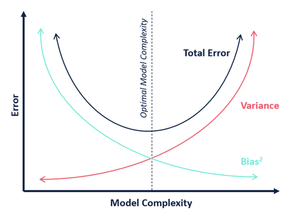
In statistics and machine learning, the bias–variance tradeoff is the property of a set of predictive models whereby models with a lower bias in parameter estimation have a higher variance of the parameter estimates across samples, and vice versa. The bias–variance dilemma or problem is the conflict in trying to simultaneously minimize these two sources of error that prevent supervised learning algorithms from generalizing beyond their training set
The bias error is an error from erroneous assumptions in the learning algorithm. High bias can cause an algorithm to miss the relevant relations between features and target outputs (underfitting).
The variance is an error from sensitivity to small fluctuations in the training set. High variance can cause an algorithm to model the random noise in the training data, rather than the intended outputs (overfitting).
The bias–variance decomposition is a way of analyzing a learning algorithm’s expected generalization error with respect to a particular problem as a sum of three terms, the bias, variance, and a quantity called the irreducible error, resulting from noise in the problem itself.
This tradeoff applies to all forms of supervised learning: classification, regression (function fitting),[1][2] and structured output learning. It has also been invoked to explain the effectiveness of heuristics in human learning.[3]
The bias-variance tradeoff is a central problem in supervised learning. Ideally, one wants to choose a model that both accurately captures the regularities in its training data, but also generalizes well to unseen data. Unfortunately, it is typically impossible to do both simultaneously. High-variance learning methods may be able to represent their training set well but are at risk of overfitting to noisy or unrepresentative training data. In contrast, algorithms with high bias typically produce simpler models that don’t tend to overfit but may underfit their training data, failing to capture important regularities.
Models with high variance are usually more complex (e.g. higher-order regression polynomials), enabling them to represent the training set more accurately. In the process, however, they may also represent a large noise component in the training set, making their predictions less accurate – despite their added complexity. In contrast, models with higher bias tend to be relatively simple (low-order or even linear regression polynomials) but may produce lower variance predictions when applied beyond the training set.
Dimensionality reduction and feature selection can decrease variance by simplifying models. Similarly, a larger training set tends to decrease variance. Adding features (predictors) tends to decrease bias, at the expense of introducing additional variance. Learning algorithms typically have some tunable parameters that control bias and variance; for example,
- linear and Generalized linear models can be regularized to decrease their variance at the cost of increasing their bias.
- In artificial neural networks, the variance increases and the bias decreases as the number of hidden units increase.[1] Like in GLMs, regularization is typically applied
- In k-nearest neighbor models, a high value of k leads to high bias and low variance (see below)
- In instance-based learning, regularization can be achieved varying the mixture of prototypes and exemplars
- In decision trees, the depth of the tree determines the variance. Decision trees are commonly pruned to control variance.[4]:307
One way of resolving the trade-off is to use mixture models and ensemble learning.[13][14] For example, boosting combines many “weak” (high bias) models in an ensemble that has lower bias than the individual models, while bagging combines “strong” learners in a way that reduces their variance.
Lost Function
In statistics, typically a loss function is used for parameter estimation, and the event in question is some function of the difference between estimated and true values for an instance of data.
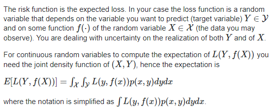
Risk Function
The risk function is the expected loss.
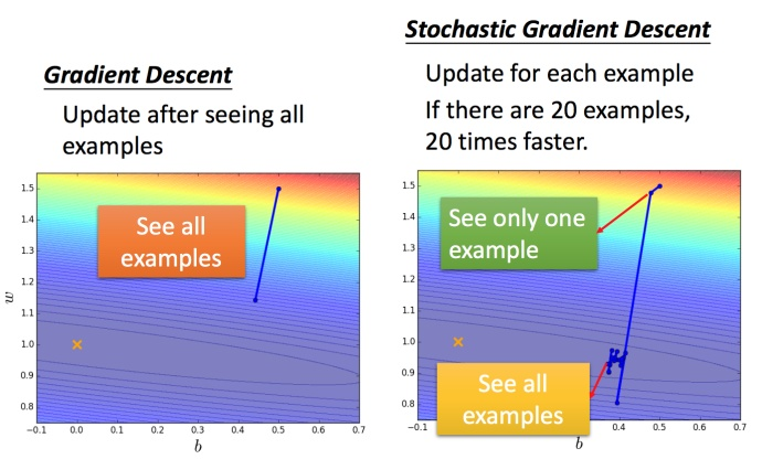
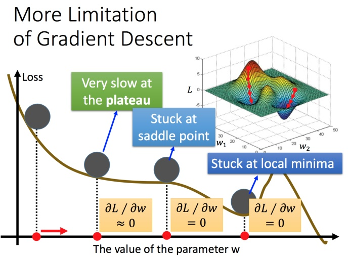
Gradient Descent
Gradient descent is a first-order iterative optimization algorithm for finding the minimum of a function (Partial derivative). To find a local minimum of a function using gradient descent, one takes steps proportional to the negative of the gradient (or approximate gradient) of the function at the current point. If, instead, one takes steps proportional to the positive of the gradient, one approaches a local maximum of that function; the procedure is then known as gradient ascent.
Gradient descent is also known as steepest descent. However, gradient descent should not be confused with the method of steepest descent for approximating integrals.
From my understanding, a convex function is one where “the line segment between any two points on the graph of the function lies above or on the graph” / “any two points inside the graph of the function can be connected by one straight line”. In this case, a gradient descent algorithm could be used, because there is a single local minimum and the gradients will always take you to that global minimum.
Gradient Descent Optimization Algorithms
Adagrad
Features:
Learning rate decreases as training progress. (Large in the first place, and then decrease gradually.)
It adapts the learning rate to the parameters, performing smaller updates
(i.e. low learning rates) for parameters associated with frequently occurring features, and larger updates (i.e. high learning rates) for parameters associated with infrequent features.
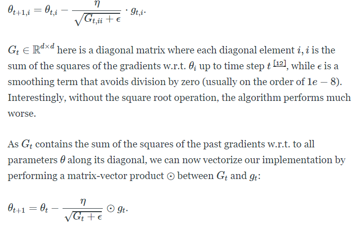
Benefits: eliminates the need to manually tune the learning rate
main weakness is its accumulation of the squared gradients in the denominator: Since every added term is positive, the accumulated sum keeps growing during training. This in turn causes the learning rate to shrink and eventually become infinitesimally small, at which point the algorithm is no longer able to acquire additional knowledge
SGD:
Feature scaling
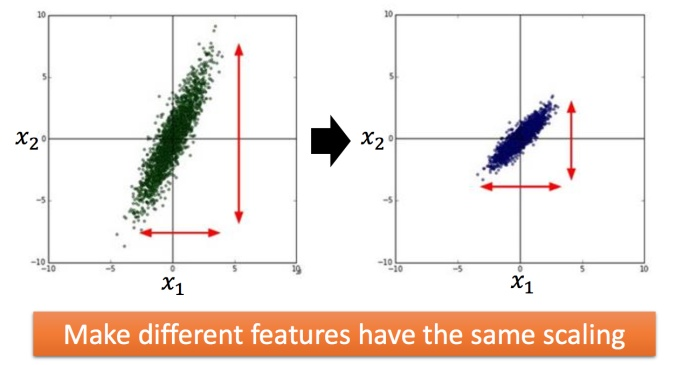
WHY?
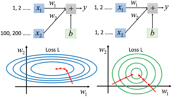
For the case on the left, the narrow and long situation was mentioned above, it is more difficult to handle without Adagrad. Different learning rates are required in both directions, and the same learning rates will not be able to handle it. In the case of on the right side, it becomes easier to update the parameters. The gradient descent on the left does not go in the direction of the lowest point, but in the direction of the tangent of the contour line. But green can go towards the center of the circle (the lowest point), so it is more efficient to update the parameters.
Gradient Descent Constraints:
May converge to local minima
Stochastic gradient descent
Backpropagation
Backpropagation algorithms are a family of methods used to efficiently train artificial neural networks (ANNs) following a gradient-based optimization algorithm that exploits the chain rule. The main feature of backpropagation is its iterative, recursive and efficient method for calculating the weights updates to improve the network until it is able to perform the task for which it is being trained.[1] It is closely related to the Gauss–Newton algorithm.
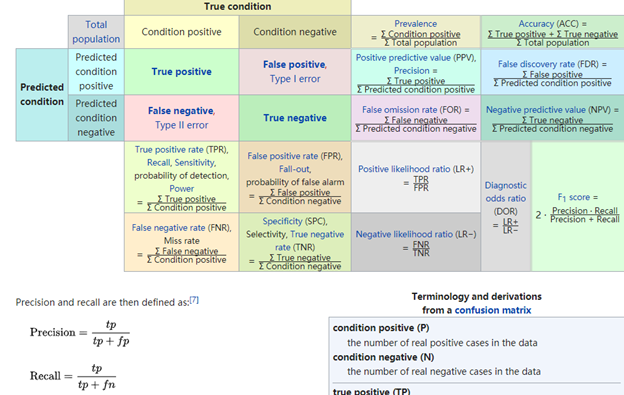
Precision and Recall
Precision means the percentage of your results which are relevant.
Recall refers to the percentage of total relevant results correctly classified by your algorithm
召回率 (Recall):正样本有多少被找出来了(召回了多少)
精确率 (Precision):你认为的正样本,有多少猜对了(猜的精确性如何)
recall expresses the ability to find all relevant instances in a dataset
precision expresses the proportion of the data points our model says was relevant actually were relevant.
Trade off
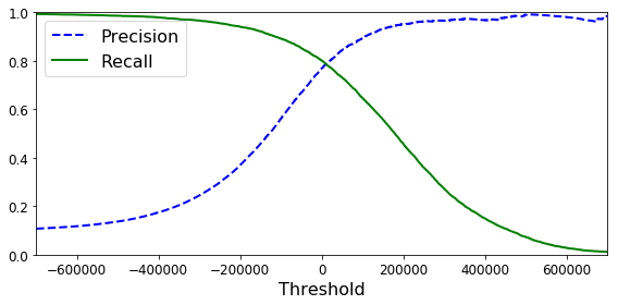
precision-recall trade-off occur due to increasing one of the parameter(precision or recall) while keeping the model same.
ROC/AUC
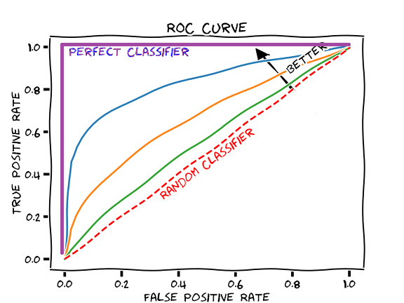
ROC is a graphical plot that illustrates the performance of a binary classifier (Sensitivity Vs 1−Specificity tp vs fp, or Sensitivity Vs Specificity tp vs tn). They are not sensitive to unbalanced classes.
AUC is the area under the ROC curve. Perfect classifier: AUC=1, fall on (0,1); 100% sensitivity (no FN) and 100% specificity (no FP)
The ROC curve is created by plotting the true positive rate (TPR) against the false positive rate (FPR) at various threshold settings. Each point of the ROC curve (i.e. threshold) corresponds to specific values of sensitivity and specificity. The area under the ROC curve (AUC) is a summary measure of performance, that indicates whether on average a true positive is ranked higher than a false positives. If model A has higher AUC than model B, model A is performing better on average, but there still could be specific areas of the ROC space where model B is better (i.e. thresholds for which sensitivity and specificity are higher for model B than A).
However, these two reasons have their own limitations, which may cause the area under the curve ** AUC ** to be less practical in some use cases:
- **It is not always desirable to keep the scale constant. ** For example, sometimes we need a well-scaled probability output, and the AUC cannot tell us this result.
- ** It is not always desirable to keep the classification threshold unchanged. ** In cases where there are large differences in the costs of false negatives and false positives, it may be important to minimize one type of classification error. For example, ** When doing spam detection, you may want to prioritize reducing false positives as much as possible (even if this results in a substantial increase in false negatives) **. For this type of optimization, the area under the curve is not a practical indicator.
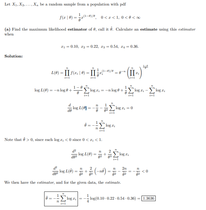
Likelihood
In statistics, the likelihood function (often simply called likelihood) expresses how probable a given set of observations is for different values of statistical parameters. It is equal to the joint probability distribution of the random sample evaluated at the given observations, and it is, thus, solely a function of parameters that index the family of those probability distributions.
Maximum likelihood estimation:
- given a pdf
-
 the pdf w.r.t X
 - Log step 2
- Get the derivate = 0 w.r.t the estimator you would like to
- Get the MLE w.r.t the estimator
pg. 4
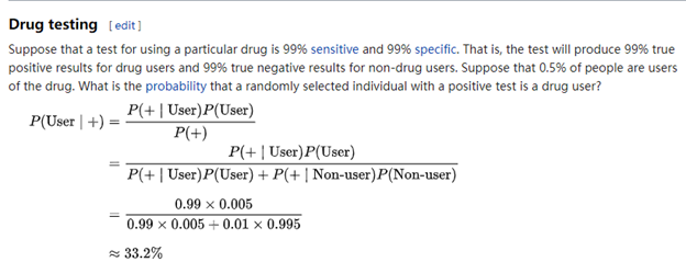
Bayes theorem
In probability theory and statistics, Bayes’ theorem (alternatively Bayes’ law or Bayes’ rule) describes the probability of an event, based on prior knowledge of conditions that might be related to the event.
Mean Squared Error Vs Mean Absolute Error
RMSE gives a relatively high weight to large errors. Since the errors are squared before they are averaged, The RMSE is most useful when large errors are particularly undesirable.
The MAE is a linear score: all the individual differences are weighted equally in the average. MAE is more robust to outliers than MSE.
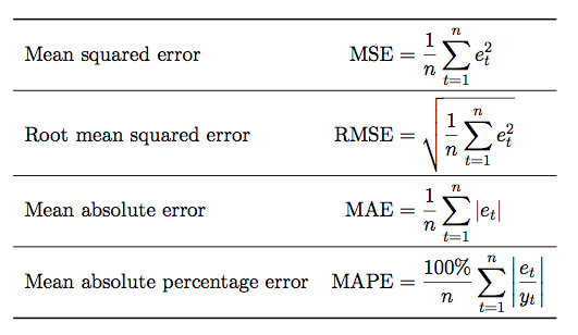
WHERE
\(e_t = y_t - \hat{y_t}\)
PCA
Assumption of logistic regression
(a) binary logistic regression requires the dependent variable to be binary and
(b) ordinal logistic regression requires the dependent variable to be ordinal.
observations should be independent of each other
little or no multi-collinearity among the independent variables
independent variables are linearly related to the log odds
ANN
A neural network is a series of algorithms that endeavors to recognize underlying relationships in a set of data through a process that mimics the way the human brain operates. Neural networks can adapt to changing input; so the network generates the best possible result without needing to redesign the output criteria.
Assumption of Linear regression
There are four principal assumptions which justify the use of linear regression models for purposes of inference or prediction:
(i) linearity and additivity of the relationship between dependent and independent variables:
1
2
3
4
5
\(a\) The expected value of dependent variable is a straight-line function of each **independent** variable, holding the others fixed.

\(b\) The slope of that line does not depend on the values of the other variables.

\(c\)  The effects of different independent variables on the expected value of the dependent variable are additive.
(ii) statistical independence of the errors (in particular, no correlation between consecutive errors in the case of time series data)
(iii) homoscedasticity (constant variance) of the errors
1
2
3
4
5
\(a\) versus time \(in the case of time series data\)

\(b\) versus the predictions

\(c\) versus any independent variable
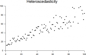
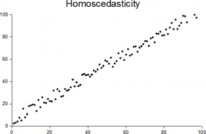
The assumption of equal variances (i.e. assumption of homoscedasticity) assumes that different samples have the same variance, even if they came from different populations. The assumption is found in many statistical tests, including Analysis of Variance (ANOVA) and Student’s T-Test. Other tests, like Welch’s T-Test, don’t require equal variances at all.
Testing for Homogeneity of Variance
Tests that you can run to check your data meets this assumption include:
(iv) normality of the error distribution.
- QQ plot
- Shapiro-Wilk
- Kolmogorov-Smirnov
- Anderson-Darling
- Correlation test
Logistic Regression
Logistic Regression, also known as Logit Regression or Logit Model, is a mathematical model used in statistics to estimate (guess) the probability of an event occurring having been given some previous data. Logistic Regression works with binary data, where either the event happens (1) or the event does not happen (0). So given some feature x it tries to find out whether some event y happens or not. So y can either be 0 or 1. In the case where the event happens, y is given the value 1. If the event does not happen, then y is given the value of 0.
Random Forest
Random forests or random decision forests are an ensemble learning method for classification, regression and other tasks that operates by constructing a multitude of decision trees at training time and outputting the class that is the mode of the classes (classification) or mean prediction (regression) of the individual trees.[1][2] Random decision forests correct for decision trees’ habit of overfitting to their training set
Features of Random Forests
It is unexcelled in accuracy among current algorithms.
It runs efficiently on large data bases.
It can handle thousands of input variables without variable deletion.
It gives estimates of what variables are important in the classification.
It generates an internal unbiased estimate of the generalization error as the forest building progresses.
It has an effective method for estimating missing data and maintains accuracy when a large proportion of the data are missing.
It has methods for balancing error in class population unbalanced data sets.
Generated forests can be saved for future use on other data.
Prototypes are computed that give information about the relation between the variables and the classification.
It computes proximities between pairs of cases that can be used in clustering, locating outliers, or (by scaling) give interesting views of the data.
The capabilities of the above can be extended to unlabeled data, leading to unsupervised clustering, data views and outlier detection.
It offers an experimental method for detecting variable interactions.
Remarks
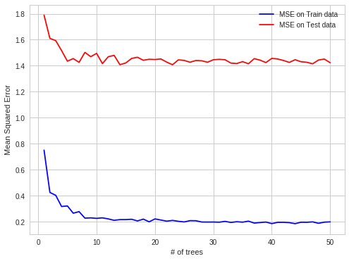
Random forests does not overfit. You can run as many trees as you want. It is fast. Running on a data set with 50,000 cases and 100 variables, it produced 100 trees in 11 minutes on a 800Mhz machine. For large data sets the major memory requirement is the storage of the data itself, and three integer arrays with the same dimensions as the data. If proximities are calculated, storage requirements grow as the number of cases times the number of trees.
Random forest does not overfit because each tree is independent and starts from scratch and Random Forest takes the average of all the predictions, which makes the biases cancel each other out. In general, more trees will be resulted in more stable generalization errors.
formula prove:
****
Learning curve
A learning curve is a graphical representation of how an increase in learning (measured on the vertical axis) comes from greater experience (the horizontal axis)
Plots relating performance to experience are widely used in machine learning. Performance is the error rate or accuracy of the learning system, while experience may be the number of training examples used for learning or the number of iterations used in optimizing the system model parameters
Collaborative filtering
Collaborative filtering (CF) is a technique used by recommender systems.[1] Collaborative filtering has two senses, a narrow one and a more general one.[2]
In the newer, narrower sense, collaborative filtering is a method of making automatic predictions (filtering) about the interests of a user by collecting preferences or taste information from many users (collaborating). The underlying assumption of the collaborative filtering approach is that if a person A has the same opinion as a person B on an issue, A is more likely to have B’s opinion on a different issue than that of a randomly chosen person. For example, a collaborative filtering recommendation system for television tastes could make predictions about which television show a user should like given a partial list of that user’s tastes (likes or dislikes)
Autoregressive Integrated Moving Average (ARIMA)
A statistical technique that uses time series data to predict future. The parameters used in the ARIMA is (P, d, q) which refers to the autoregressive, integrated and moving average parts of the data set, respectively. ARIMA modeling will take care of trends, seasonality, cycles, errors and non-stationary aspects of a data set when making forecasts.
Decision Tree or Logistic Regression
Both decision trees (depending on the implementation, e.g. C4.5) and logistic regression should be able to handle continuous and categorical data just fine. For logistic regression, you’ll want to dummy code your categorical variables.
As @untitledprogrammer mentioned, it’s difficult to know a priori which technique will be better based simply on the types of features you have, continuous or otherwise. It really depends on your specific problem and the data you have. (See No Free Lunch Theorem)
You’ll want to keep in mind though that a logistic regression model is searching for a single linear decision boundary in your feature space, whereas a decision tree is essentially partitioning your feature space into half-spaces using axis-aligned linear decision boundaries. The net effect is that you have a non-linear decision boundary, possibly more than one.
This is nice when your data points aren’t easily separated by a single hyperplane, but on the other hand, decisions trees are so flexible that they can be prone to overfitting. To combat this, you can try pruning. Logistic regression tends to be less susceptible (but not immune!) to overfitting.
Lastly, another thing to consider is that decision trees can automatically take into account interactions between variables, e.g. xy if you have two independent features x and y. With logistic regression, you’ll have to manually add those interaction terms yourself.
So you have to ask yourself:
what kind of decision boundary makes more sense in your particular problem?
how do you want to balance bias and variance?
are there interactions between my features?
Of course, it’s always a good idea to just try both models and do cross-validation. This will help you find out which one is more likely to have better generalization error.